Curve Fitting
EZL computes curve fits as least squares polynomial equations. Ill-conditioned data are handled by pre-removing the mean of the independent variable before computing an LU decomposition. This results in numerically accurate curve fits, even for high orders models. The polynomial equations can either be printed to the Command Window, or used directly to detrend your curves.
Curve fitting functions in EZL are accessed either through the Curve Fitting Toolset, or via the poly command.
The Curve Fitting Toolset
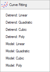
The Curve Fitting Toolset provides quick access to the two primary operations, Detrend and Model. For each operation, the toolset provides quick access to linear, quadratic, and cubic order fits (1st, 2nd, and 3rd order, respectively), and a poly option which allows you to specify higher order fits.
Use of the toolset options result in operations involving all curves on the active plotter. To operate on individual curves, see the section on The Poly Command.
Detrend
Clicking on any of the quick-access detrend options, Detrend: Linear, Detrend: Quadratic, or Detrend: Cubic, will immediately compute a corresponding polynomial curve-fit for each of the curves on the plotter. The curve-fit equation(s) will then be used to automatically detrend the curve(s).
Clicking on the Detrend: Poly option will first prompt you to enter a polynomial order. A polynomial curve-fit of the given order will then be immediately computed and used to detrend the existing curves.
Model
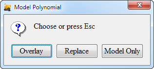
The Model options are used to provide you with curve-fit equations without actually modifying your existing curves. When modeling curve-fit equations, you have three additional options:
- Overlay - This option draws the computed curve-fit polynomials on the plotter as new curves. The polynomial curves therefore overlay, or, are drawn on top of, the existing curves, providing you with an easy way to judge the accuracy of their approximations.
- Replace - Similar to Overlay, except now the existing curves are replaced with their polynomial fits.
- Model Only - Selecting this option will make no modification to the curves on the plotter.
For all Model options, the resulting polynomial equation(s) will be printed to the Command Window.
As with Detrend, the Curve Fitting toolset contains Model quick-access buttons for Linear, Quadratic, and Cubic polynomials. And, as before, it contains a Model: Poly option for manually specifying the polynomial order.
The Poly Command
The poly command provides you with all of the functionality of the Curve Fitting Toolset, but also always you to operate on individual curves in the plotter. The syntax is as follows, as reported by the "help poly" command:
> Format : Poly<n> [{model|overlay*|replace|detrend}] [Cj]
> Purpose : Polynomial curve fitting.
> Options : n - order of polynomial (required).
> "model" - Instructs ezl to write the polynomial equation to the command window,
and not plot the polynomial curve (optional enumeration).
> "overlay" - Instructs ezl to plot the polynomial on top of the original data, as
a new curve. The equation will also be written to the command window.
This is the default enumeration option.
> "replace" - Replaces the original data with the polynomial curve. The equation will
also be written to the command window.
> "detrend" - Removes the nth order polynomial equation from the specified curves.
> Cj - Indicates a selection of curves on which to operate.
As described by the report of "help poly", the command begins with
poly<n>, where n is the polynomial order.
So, poly1 will generate a 1st order equation:
a1x + a0
poly2 will generate a 2nd
order equation: a2x2 + a1x + a0
poly3 will generate a 3rd
order equation: a3x3 + a2x2 +
a1x + a0
and so on...
Following the poly<n> syntax is the optional operation type: model, overlay*, replace, or detrend. The * next to overlay indicates that this is the default operation mode. If no operation is specified, the command will use overlay.
The next optional parameter, Cj may be used to indicate which curves should be included in the operation. This parameter is specified as a list of curve identifiers, such as: c1 c2 c4 c5.
Poly Command Examples:
| poly1 detrend | This command will remove the 1st order (linear) fit of each curve on the plotter. In the absence of a Cj list, all curves are included by default. |
| poly10 detrend c2 | This command will remove the 10th order fit of curve C2. |
| poly10 overlay c2 c5 | This command will model the 10th order fits of curves C2 and C5, and create two new curves representing their fitted polynomial equations. |
| poly10 c2 c5 | Same as above. The "overlay" option is the default mode. |
| poly2 model | This command will model the quadratic fits of all curves on the plotter. The modeled polynomial equations will be displayed on in the Command Window. |
Curve Fitting Demo
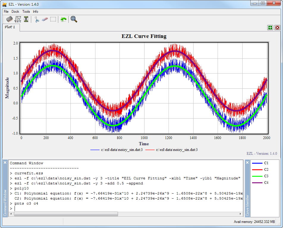
As a demonstration of curve fitting in EZL, consider the following EZScript:
--> An example script to demonstrate curve fitting
ezl -f c:\ezl\data\noisy_sin.dat -y 3 -title "EZL Curve Fitting" -xlbl "Time" -ylbl "Magnitude"
ezl -f c:\ezl\data\noisy_sin.dat -y 3 -add 0.5 -append
poly10
pnts c3 c4
The first line of the script (ignoring the comment line) plots column 3 from a file named "noisy_sin.dat", and sets the title, x-axis label, and y-axis label. The data contained in this file comprises a simple sine wave with noise superimposed.
The second line, for simplicity, re-plots the same data with a y-offset of 0.5. We use the -append flag in order to prevent the previous curve from being cleared.
The third line, poly10, creates a 10th order polynomial with the default options - which includes all curves on the plotter and specifies the "overlay" operation mode.
The final line enables the point markers for curves C3 and C4 so that these curves are more visible for the demo. Notice that curves C3 and C4 do not exist until after the third line is executed, as it is the poly10 command which creates them.
The results are displayed below.