Data Filtering

The EZL toolsets panel displaying the filters toolset.

There are multiple ways to filter, smooth, and average data in EZL. Aside from the Smooth Command, these operations are accessed through the Filters toolset (see the image on the right).

The first two, Average Data and Average Data Span are used to combine (average) multiple data points into single values.

The others allow you to create and apply digital filters to your data. All three Smooth Data, IIR, and FIR, open EZL's filter design tool when clicked.

Average Data

The Average Data function bin-averages n points of an existing curve, producing a new curve with j/n points, where j is number of points in the original curve.

For example, suppose you average 100 points, given a 5000 point curve. The first point of the new curve will be the average of the first 100 points of the original curve. The second point will be the average of the next 100 points, and so on. The final curve will therefore consist of 50 points.

Just as the the y-axis values are averaged to produce the new ordinate values, the x-axis values are similarly averaged to yield the new coordinates' abscissa values. For example, if our first 100 points are evenly spaced from 0 to 99, the new averaged data point will be placed at 49.5.

When the Average Data button is first clicked, a simple prompt will open requesting the number of points to use for the average. Following this, a second prompt will be displayed asking if you would like the new curve to be overlayed or not. Select yes to add the new curve to the plotter, leaving the existing curve in place. Select no to replace the original curve with the new averaged curve. Finally, if you currently have more than one curve on the plotter, a third prompt is displayed allowing you to indicate which of the existing curves should be operated upon.

Average Data Span

The Average Data Span function is similar to the Average Data function described above, except that whereas with Average Data you specify a fixed number of points for the average, here you specify a fixed span of data.

For example, suppose your curve consists of daily measurements starting on Day 1 and ending on Day 100. You want to average the values across each day, but each day does not necessarily have an equal number of measurements. In this case, you would use the Average Data Span function, and specify a span of 1, assuming your data is plotted from MJD, ASCII timestamps - which internally is converted to MJD, or another fractional day representation. Or, if your data is plotted in seconds, where the first point is the first second of Day 1, you would set the span to 86400 (the number of seconds in a day).

Smooth Data

The Smooth Data function is part of the digital filter set. Please see the Filter Design section for details.

The Smooth Command

Arguably one of the the most commonly used filtering tools within EZL is the smooth command. This command provides a fast, simple way to smooth your data curves from directly within the Command Window. Typing "help smooth" within the Command Window provides usage details

> help smooth

> Format  : Smooth <n> [Cj] [{overlay|replace*}]

  Purpose : Smooth curve(s) Cj by n points.

  Options : [Cj] - Optional list of curves to smooth (ex. C1 C3)

            "overlay" - instructs ezl add the smoothed results to the plot as new curves.

            "replace" - (default) instructs ezl to replace the existing unsmoothed curves.

                        with the new smoothed results.

  Example : "smooth 15" smooths all curves by 15

            "smooth 15 C1 C2" smooths curves C1 and C2 by 15

            "smooth 10 C1 overlay" smooths curve C1 by 10 and add results as a new curve

IIR - Infinite Impulse Response

The IIR function is part of the digital filter set. Please see the Filter Design section for details.

FIR - Finite Impulse Response

The FIR function is part of the digital filter set. Please see the Filter Design section for details.

Filter Design

As the name suggests, the Filter Design tool allows you to generate custom digital filters to apply to your data.

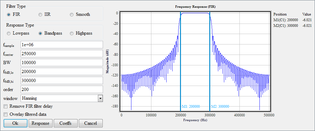
As shown in the image, you can choose between Finite Impulse Response (FIR), Infinite Impulse Response (IIR), and Smoother filter types. For FIR and IIR types, you can select Lowpass, Bandpass, and Highpass responses (smoother filters are lowpass by nature).

Filter specifications:

f_sample - This is the sample frequency of the data. It is equal to the reciprocal of the sample period, 1/T. This field is automatically populated based on the data currently plotted, but you can modify it as needed.
f_center - For bandpass filter types, this is the center frequency of your filter. When designing bandpass filters, you can either specify the filter's center frequency and its bandwidth, or the low and high cutoff frequencies.
BW - For bandpass filter types, this is the filter's bandwidth. When designing bandpass filters, you can either specify the filter's center frequency and its bandwidth, or the low and high cutoff frequencies.
f_dB,lo - For bandpass filter types, this is the filter's low cutoff frequency. For IIR filters, it is specified as a 3dB point. For FIR filters, it is specified as a 6dB point.
f_dB,hi - For bandpass filter types, this is the filter's high cutoff frequency. For IIR filters, it is specified as a 3dB point. For FIR filters, it is specified as a 6dB point.
f_dB - For lowpass and highpass filter types, this is the filter's low or high cutoff frequencies, respectively. For IIR filters, it is specified as a 3dB point. For FIR filters, it is specified as a 6dB point.
order - The order of the filter.
window - For FIR filters, the following window functions are available
- Bartlett (aka Triangular)
- Blackman
- Boxcar (aka Rectangular)
- Hamming
- Hanning
- Welch
- Need Another? Ask us!

Below the filter specification fields are two checkboxes:

Remove FIR filter delay - Applicable to FIR filters only (which are phase linear), this option instructs EZL to undo the delay from the data after filtering. It essentially allows the filter to behave as a zero-phase filter.
Overlay filtered data - Check this box to overlay the new filtered curves onto the plotter, without deleting the original (unfiltered) curves from the plotter. Leave the box unchecked to replace the existing curves with the new filtered results.

Once you have entered the filter parameters, you can view the filter response by clicking on the Response button. If desired, you can zoom-in on portions within the filter response plot, by drawing a box around the zoom area, just as you normally would do for any EZL plot. To rescale back to full-view, simply click the Response button again.

You can view the filter's coefficients, by clicking the Coeffs button. Doing so will popup a window like the example below:

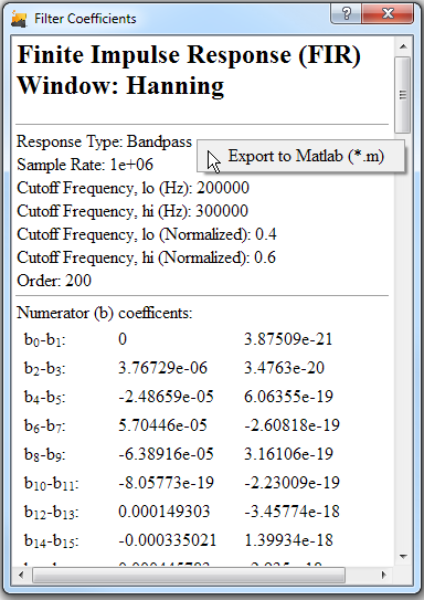
The filter's coefficients is easily exported. Displayed here are the specifications of a bandpass FIR filter with a Hanning window.

To export the coefficients to an easy to use MATLAB® .m script, simply right-click anywhere within the coefficients page and select "Export to Matlab."

Finally, to apply your filter to the curves, simply click "Ok". Remember, you can always type "undo" in the Command Window if you are unsatisfied with the results and would like to try again!

*Suggestion - Save for the simple case of a smoother filter, it is recommended to view the frequency spectrum of your data (Toolsets -> Power Spectral Density) before creating your filter. This helps you determine the best placements for your cutoff frequencies!